
Sometimes if you have copied and pasted data from a different source e.g. a web page/ an e-mail/another document, you might find yourself with broken formulae or rogue characters in your lists of data that you don’t want. Some of the following techniques (or a combination of them!) may help.
TRIM
If your data visually looks correct but your formula isn’t working, check for additional spaces. By double clicking the cell you can arrow left and right through the characters to check for extra spaces. Alternatively you can use a LEN formula to see if the length of the cell (the number of individual characters in the cell) is the same as what you visually count. If by these investigations you discover additional spaces where you don’t want them (e.g. 2 spaces between words, or an extra space at the begging or an extra space at the end) and then discover the same thing is happening all the way down your dataset – fear not! You won’t have to go through every single cell manually one by one to remove them! Instead use TRIM. You’ll love it!
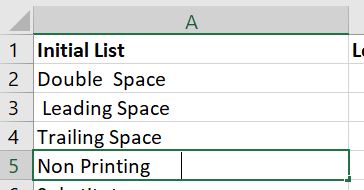
Below is an example of 3 types of extra space that TRIM can remove
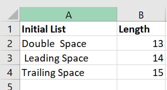
I have included in column B the LEN formula which is counting the number of characters in that cell. In each case there is one too many characters – either a double space, a space at the start or a space at the end.
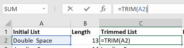
To remove these spaces in a fresh column type in =TRIM(
Then select the cell in column A that you want to remove the extra spaces from then close the bracket with ) and hit Enter
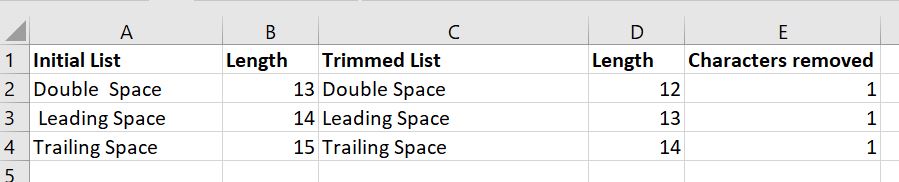
The result will be the same cell but with additional spaces removed. I have done this on all three examples by copying the formula down, and in column D I’m showing a fresh LEN formula to prove that the length of the cell is now one less as the additional space has been removed.
Then you can either reference your new Trimmed column in your next formula (recommended if the source data will be regularly updated and the exercise repeated!), or copy and hardcode paste your freshly trimmed dataset over the original list and remove all the extra formulas so you’re back to a nice Trimmed dataset and can carry on.
CLEAN
Sometimes TRIM isn’t enough. TRIM will only work on normal characters. However sometimes your dataset will secretly be harbouring “non-printing characters”.
In the below example on row 5 you will see that TRIM did not remove any characters, but there are too many in the cell – there should be 12 characters (3, then 1 space, then 8) not 13.
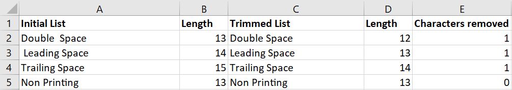
If I double click in the cell you will see one large space after the word printing which must be what is being recognised as the thirteenth character
So this this situation, instead of (or in addition to TRIM by nesting TRIM) we will use CLEAN.
To use CLEAN in a fresh column type in =CLEAN(
Then reference the cell that you want to clean then close the bracket with ) and hit Enter.

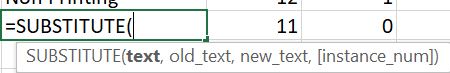
If neither of those methods work your last option may be the Substitute formula.
To use substitute you need to
- first reference the cell with the data “text”
- then indicate the character or word that you want to remove “old_text”
- then indicate the character or word that you want to replace it with – this might simply be nothing
- then if it appears several times you may want to indicate which instance of the old text you want to replace.
Whilst Substitute is very powerful, it depends on you knowing exactly what the bad character is in your dataset to be able to swap it out. However it’s a helpful formula to be aware of if you are in a sticky situation like this when cleaning your dataset.