
If you’ve inherited an Excel file you may have looked at the formulae and seen lots of $ signs all over it and wanted to run away in fear. Don’t worry! It’s not as scary as it looks once you understand what it’s for!
Usually the dollar sign $ in the formula is not about currency (with the exception of format formulas but more on that another time!). The dollar sign $ is actually a way of locking a part of your formula to a column and/or row so that when you drag the formula down or right the part of the formula you want locked stays put and your formula doesn’t break (essential for future proofing). This is actually, in my experience, one of the most common mistakes made when trying to write your own formulas and in a hurry. I will explain how this dollar sign $ works but first you must know this trick….
Instead of writing the dollar sign $ in your formula you can hit the function button F4 button on your keyboard at the right time when writing your formula. Below I will explain how to use this alongside understanding what the dollar sign $ does in your formula.
Pro Tip: If pressing F4 doesn’t work when you try the below guide, check you have the function buttons on on your keyboard. Sometimes you need to hold down an FN button to press Function keys or lock FN on – a bit like with CAPS Lock with a small “on” light on your keyboard. I personally use the F4 button all the time in Excel so I like to have the FN functions on pretty permanently. If you will be using Excel heavily and writing formulas it’s a good idea to lock this in permanently too. If you can’t see a button with a light on your keyboard you might need to hold both the FN key and the Caps Lock key to lock the Function keys on (and do the same again if you want to switch them off at a future date). Or if you are lucky and have a full standard keyboard hopefully you have your Function keys entirely separate anyway so you are all good. 🙂
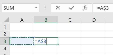
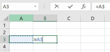
I’ve opened a blank Excel file and I’m in cell B3 just to demonstrate, so feel free to follow along and do the same

When writing a formula from scratch (anything with an “=” at the start in a cell!), after selecting the cell you want to reference in your formula, hit F4 once. In above image I selected cell A3 then hit F4 on my keyboard. Automatically Excel has inserted a dollar sign $ before the letter A and a dollar sign $ before the number 3 and left the cursor where it was where I was writing so I can carry on writing my formula without interruption. What this has done is lock both column A and row number 3 into that cell reference in the formula. The magic then is that if I finish writing my formula and enter it, then drag or copy and paste the formula elsewhere in my spreadsheet, it will still be referencing cell A3. So if I had something important in there that I only wanted to change once and have all my formulas feed off that once cell, this is how you can use it e.g. if I wanted to type in a price and have lots of formulas calculate the total price at lots of different volumes across my spreadsheet.
If instead you pressed the F4 button twice Excel will lock the Row number only by putting the dollar sign $ only in front of the number 3. In this case if I copy my formula elsewhere it will change the Column number to the relevant cell wherever my new formula is located.
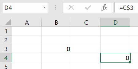
For example if I moved the formula to cell D4 it would be referencing column C (the one just to the left of my formula cell, just like how A3 is just left of the B3 – my formula cell). However it will still keep the row number as 3 so I would end up with C3. Take a moment to get your head around that before moving on.
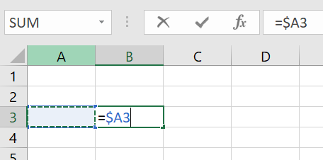
If instead you pressed the F4 button three times Excel will lock the Column letter only by putting the dollar sign $ only in front of the letter A. In this case if I copy my formula elsewhere it will change the row to the relevant cell wherever my new formula is located.
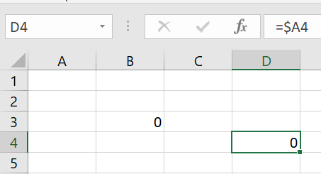
For example if I moved the formula to cell D4 it would still be referencing column A as that is the one it’s locked to, but the row number would have moved from 3 to 4.
If you press F4 four times it basically resets back to an unlocked cell reference so you can start again if you accidentally went past the option you wanted. Alternatively instead of pressing F4 you can manually go into the formula and pop in the dollar sign $ where you need it, just remember to put the cursor back to the end of the formula when you’re done.
Timing of using F4 is also important when writing your formula. If you’ve already written a comma in your formula then you’ve closed off the part of the formula you might have wanted the dollar signs $ to appear on so remember to work out what you want to lock in your formula before you move on with writing. This is where thinking ahead about where you will want to copy and paste your formula next and good spreadsheet design is key.
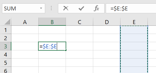
Also if you are selecting a range of cells, you only need to (and can only) press F4 once and it will lock the relevant row or column. As you can see there’s only the column or row referenced (in this case column E) so Excel doesn’t need to give you lots of different options for combinations of dollar signs. So in this case pressing F4 twice resets it back to the start clean reference.
Using F4 with Shift or with Ctrl can do different things so ensure you are not holding either of those two buttons at the same time.
And you’re done with learning about what the dollar sign $ is for in a formula. Mastering this and using it correctly and regularly will help make sure your spreadsheets don’t break as they evolve, and speed up your spreadsheet making. It’s a super powerful tool in Excel and will have you feeling like a whizz in no time!
Have fun with F4!