
Basic Excel
When to use VLOOKUP
There are two important causes that trigger the need for this formula.
- You have two different datasets and you need to combine data from both of them (e.g. A list of products in one and a summary of stock levels by product in another), AND
- both datasets already have a common field with identical values that are unique in both lists (e.g. Product ID codes).
And you don’t want to manually visually look at both lists on the screen or on paper and match things up one by one as that would take an age!
Pro Tip: If you don’t have a common field with identical values, there are ways around this – check out some ideas about how to obtain this (FORTHCOMING)
How to use VLOOKUP
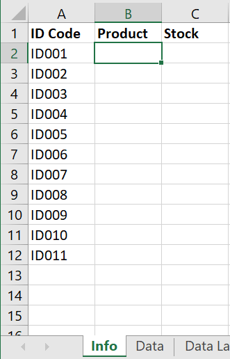
In this example I have two datasets within one excel file, one called Info and one called Data.
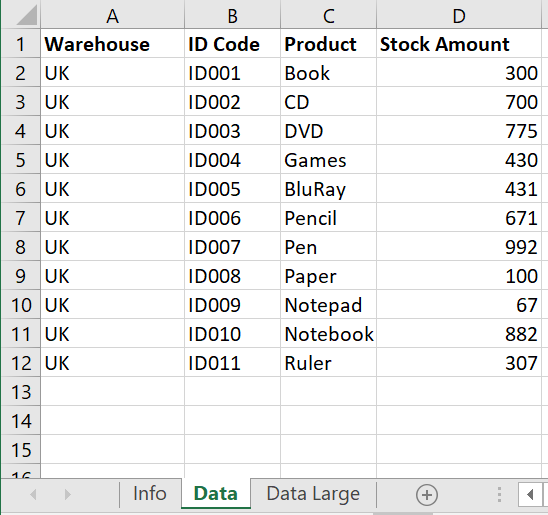
Whilst the Data tab has lots of useful data, it is split up by warehouse (and possibly lots of other columns which we can’t see). As a result there are potentially a lot of rows with repeated identical information per row, with the only difference being the warehouse – and you may have many hundreds of sets of these!
If you are tasked to summarise this dataset to show in Total what the stock levels are per Product in a small neat table as specified in the Info tab – something nice to use in a nice report or presentation, that is what we will put on the Info tab.
There are lots of ways to do this. For example you could filter on one product at a time and add up the numbers manually/visually/with a formula, or you could use a pivot table (a very good alternative approach for such a task, but not the focus of this post!). However in this tutorial we will look at using a VLOOKUP formula – one of the most invaluable basic Excel formulae.
VLOOKUP – one of the most invaluable basic Excel formulae
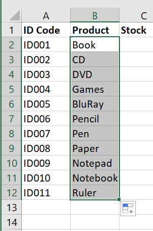
So in Column B of the Info tab I want to write a formula to bring back the name of the Product the Product ID relates to so it is easier to read, digest and understand (as it is likely the end user of the summary will not know which Product ID is which!).
Pro Tip: it is good to always apply a VLOOKUP against a code or number ID from a pair of data, rather than the description or name of that ID. This is because whilst the name of an ID may inevitably change (e.g. it may have originally be mistyped or the name of a product needs extra info added as an after thought etc.) it is likely the number itself will not change so the table within which you are trying to summarise the data will still work even if the product name is changed at a later date. This is very useful if you are likely to update the source data in the Data tab and want to recycle your summary formula. It’s a good way to future proof your formula and is a good habit to get used to right away.
Type =VLOOKUP(
Pro Tip: When you start typing in =vlo Excel will also try to predict what you are trying to do and suggest it in an automatic drop down. Instead of finishing what you are typing you could double click what it suggested if it is what you want and Excel will automatically finish typing in VLOOKUP( including the open bracket. See below:

Then select (or type in) the single cell in the column you want to reference – in this case A2 (you can simply point and click the cell). Hit F4 on your keyboard 3 times to automatically add a $ in front of the column letter to lock the formula to that column, then type in a comma ,
So you should have =VLOOOKUP($A2,
Then you need to choose the range of cells or columns of the dataset, or table, that you want to reference. What is most important is that the column that will have values that match your reference column, is the left most column of your selected dataset.
Pro Tip: The column that has the values that match your reference column MUST be the first column of your selected dataset for a VLOOKUP to work, but it doesn’t matter if there are columns before it, as long as you won’t need them later on. If it’s not the first column you may need to cut and paste the column to the left of the data you will need or alternatively (which I strongly recommend), use INDEXMATCH formula instead (GUIDE FORTHCOMING!) to avoid manually manipulating the dataset you are referencing. This is good practice if this is a task you might repeat regularly and the dataset you reference will need to be easily updated with fresh data in future (e.g. a dataset you download from a reporting tool or receive by e-mail) or you need to write a new VLOOKUP formulae to reference different columns and bring back other ones. So be smart about it if in those situations and embrace INDEXMATCH (it’s just a fancier and smarter VLOOKUP) or alternatively Excel’s brand new XLOOKUP (though this won’t be backward compatible yet so don’t use that if your file users have older versions of Excel)
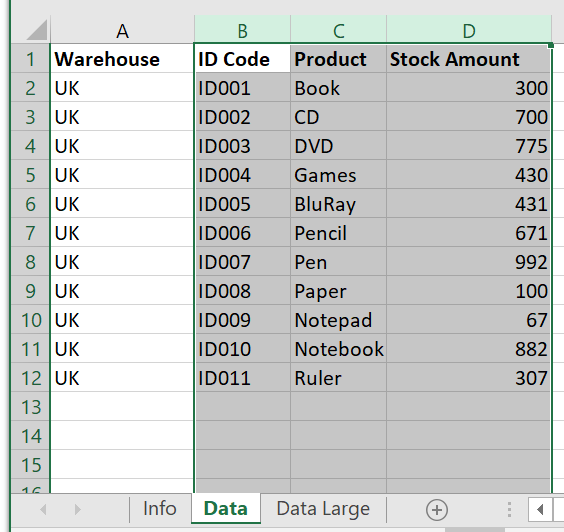
In our example, after typing in the comma before, then select the Data tab and highlight the full columns from B to D. Then hit F4 once to lock in those columns (when selecting entire columns you only need to hit F4 once). Then type in a comma ,
Pro Tip: There are lots of different ways to select your dataset range. If you select the entire column in this way it future-proofs the formula so if at a later date you update the Data tab with more data or more rows the formula will still work without needing editing. If you only selected the cells then the formula will not automatically pick up any new data unless you manually edit the formula to cover the new range entirely – it’s therefore good to avoid this issue. However the caveat is that in very large excel files referencing an entire column may require heavy computer memory usage and slow down your file. If you get to that stage with a huge amount of data and a formula heavy file, it’s better to use an Excel Table format instead (GUIDE FORTHCOMING) to save memory hungry requirements of your file.
Pro Tip: Notice also that when you moved to the second tab the formula automatically wrote in “Data!” to recognise that you moved tabs. Keep an eye on when Excel does this. Sometimes it can write in the name of the tab when you don’t want it to, so if you copied the formula somewhere else it would still be referencing that tab – sometimes you want it to do that sometimes you don’t so be consciously aware when it has done that. If you clicked back to the Info tab without typing in a comma during this formula, it will suddenly change the tab reference to Info tab instead of the Data tab and your formula will be broken (try it and see!). So typing in comma at the right time when writing a formula is very important as it ends that section of the formula. If the formula has gone wrong and you can’t recover it, hit ESC on your keyboard to exit the cell and start again. Trust me though, it will become habit with practice. 🙂
So you should now have =VLOOKUP($A2, Data!$B:$D,
That’s the hard bit done. Now it’s easy.
Next step is to tell the formula which column you want it to bring back when it’s matched your reference cell. The first column of your range dataset if always column number 1 – in this case column B. So then count the number of columns from the first column of your range dataset and work out the column number you want it to bring back. In this case we want column number 2 (Column C – the next column after B) which had the Product name. So type in 2 and then type in a comma ,
Pro Tip: For huge datasets you might want to insert a row at the top and type in the column numbers 1, 2, 3 etc. from your chosen column 1 for easy visual reference rather than visually counting on the screen as you won’t be able to scroll to the right of a sheet mid formula writing without the formula breaking. There are also many other tips and tricks here that you could learn to enhance the efficiency of writing a VLOOKUP for example referencing a cell with the number in it rather than hardcoding the number 2 in your formula, or using a formula to dynamically work out the column number (GUIDE FORTHCOMING!). But pace yourself, you will learn those tricks in time!
And finally, type in FALSE then close the bracket with ). Then hit Enter on the keyboard and the formula completes and you exit the cell. Woop!
Pro Tip: I know, it’s weird to write FALSE. This is asking if you want it to roughly match your reference cell or to exactly match your reference cell. To roughly match you write in TRUE or to exactly match you write in FALSE. In almost all cases you usually need it to match exactly so you write in FALSE. Very very very rarely will you need TRUE and in my personal experience I think I’ve only ever used it once…if that…
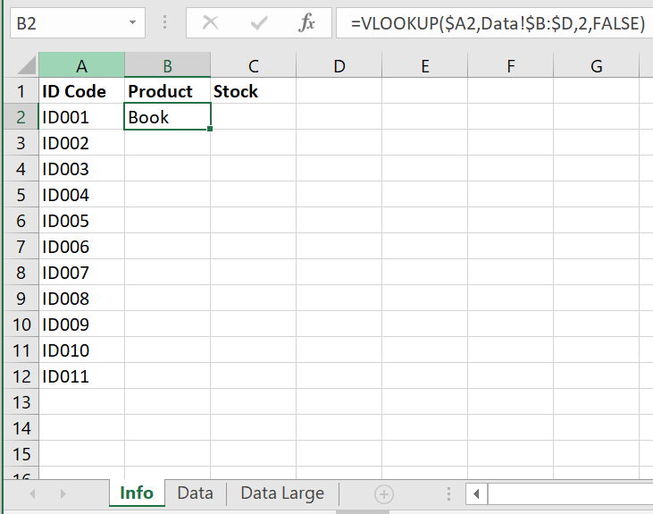
So finally you end up with the below
=VLOOKUP($A2,Data!$B:$D,2,FALSE)
If all is well you should now have the result you were expecting in the cell. Visually sense check your formula and results to ensure you are happy that it worked.
When you are happy with this you can copy your formula down the column. Either manually copy and paste down using keyboard shortcuts or right clicking and copy and pasting, or my favourite method, hovering over the bottom right corner of the cell and double clicking and you see a black cross appear. Then Excel will automatically copy the formula all the way down the column whilst there is data in the column before it. If your data has a gap (an empty cell) or stops the formula will stop too.
Once this is done again double check it worked as expected. If you haven’t locked the columns or rows properly it might not work so check carefully and inspect a few formulas below the one you wrote (learn more about locking cell reference soon (see What are all the $ signs for) guide
And voila you’ve used a VLOOKUP formula.
Well done! 😀
The VLOOKUP is one of the most commonly used formulae with lots of ways of adapting it and using it to accommodate lots of different uses so keep using it and be inventive using all the tips and tricks you learn such as locking cells etc. The more you use it the more you’ll master it and be teaching others before you know it!
Happy VLOOKUPing!